Visualising the predictive distribution of a log-transformed linear model

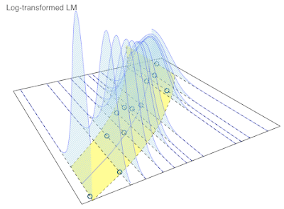
Last week I presented visualisations of theoretical distributions that predict ice cream sales statistics based on linear and generalised linear models, which I introduced in an earlier post.

Theoretical distributions

Today I will take a closer look at the log-transformed linear model and use Stan/rstan, not only to model the sales statistics, but also to generate samples from the posterior predictive distribution.

The posterior predictive distribution is what I am most interested in. From the simulations I can get the 95% prediction interval, which will be slightly wider than the theoretical 95% interval, as it takes into account the parameter uncertainty as well.

Ok, first I take my log-transformed linear model of my earlier post and turn it into a Stan model, including a section to generate output from the posterior predictive distribution.


After I have complied and run the model, I can extract the simulations and calculate various summary statistics. Furthermore, I use my parameters also to predict the median and mean, so that I can compare them against the sample statistics. Note again, that for the mean calculation of the log-normal distribution I have to take into account the variance as well.


Ok, that looks pretty reasonable, and also quite similar to my earlier output with glm. Using my plotting function of last week I can also create a nice 3D plot again.

Posterior predictive distributions

Just as expected, I note a slightly wider 95% interval range in the posterior predictive distributions compared to the theoretical distributions at the top.

Session Info

R version 3.2.2 (2015-08-14)
Platform: x86_64-apple-darwin13.4.0 (64-bit)
Running under: OS X 10.10.5 (Yosemite)

locale:
[1] en_GB.UTF-8/en_GB.UTF-8/en_GB.UTF-8/C/en_GB.UTF-8/en_GB.UTF-8

attached base packages:
[1] stats     graphics  grDevices utils datasets 
[6] methods   base     

other attached packages:
[1] rstan_2.7.0-1 inline_0.3.14 Rcpp_0.12.0  

loaded via a namespace (and not attached):
[1] tools_3.2.2 codetools_0.2-14 stats4_3.2.2

Posted by Unknown

Tweet