Bayes' theorem
Bayes' theorem states that given two events \(D\) and \(H\), the probability of \(D\) and \(H\) happening at the same time is the same as the probability of \(D\) occurring, given \(H\), weighted by the probability that \(H\) occurs; or the other way round. As a formula it can be written as:\[
P(H \cap D) = P(H|D) \, P(D) = P(D|H) \, P(H)
\]
Or if I rearrange it:
\[
P(H|D) = \dfrac{P(D|H) \, P(H)}{P(D)}
\]
Imagine \(H\) is short for hypothesis and \(D\) is short for data, or evidence. Then Bayes' theorem states that the probability of a hypothesis given data is the same as the likelihood that we observe the data given the hypothesis, weighted by the prior belief of the hypothesis, normalised by the probability that we observe the data regardless of the hypothesis.
The tricky bit in real life is often to figure out what the hypothesis and data are.
Hit and run accident
This example is taken from Daniel Kahneman's book Thinking, fast and slow [1].A cab was involved in a hit and run accident at night. Two cab companies, the Green and the Blue, operate in the city. 85% of the cabs in the city are Green and 15% are Blue. A witness identified the cab as Blue. The court tested the reliability of the witness under the same circumstances that existed on the night of the accident and concluded that the witness correctly identified each one of the two colours 80% of the time and failed 20% of the time.
What is the probability that the cab involved in the accident was Blue rather than Green knowing that this witness identified it as Blue?
What is here the data and what is here the hypothesis? Intuitively you may think that the proportion of Blue and Green cabs is the data at hand and the witness accusation that a Blue cab was involved in the accident is the hypothesis. However, after some thought I found the following assignment much more helpful, as then \(P(H|D)\) matches the above question:
\(H =\) Accident caused by Blue cab. \(D =\) Witness said the cab was Blue.
With this it is straightforward to get the probabilities of \(P(H)=15\%\) and \(P(D|H)=80\%\). But what is \(P(D)\)? Well, when would the witness say that the cab was Blue? Either, when the cab was Blue and so the witness is right, or when the cab was actually Green and the witness is incorrect. Thus, following the law of total probability:
$$\begin{align}
P(D) & = P(D|H) P(H) + P(D | \bar{H}) P(\bar{H})\\
& = 0.8 \cdot 0.15 + 0.2 \cdot 0.85 = 0.29
\end{align}$$Therefore I get \(P(H|D)=41\%\). Thus, even if the witness states that the cab involved in the accident was Blue, the probability of this being true is only \(41\%\).
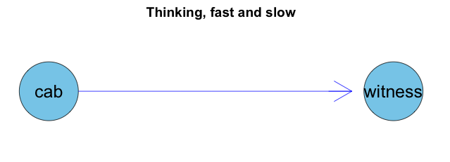
An alternative way to think about this problem is via a Bayesian Network. The colour of the cab will influence the statement of the witness. In R I can specify such a network using the gRain package [2], which I discussed in an earlier post. Here I provide the distribution of the cabs and the conditional probabilities of the witness as an input. After I compile the network, I can again read off the probabilities that a Blue cab was involved, when the witness said so.
R code
References
[1] Daniel Kahneman. (2011). Thinking, Fast and Slow. New York : Farrar, Straus and Giroux.[2] Søren Højsgaard (2012). Graphical Independence Networks with the gRain Package for R. Journal of Statistical Software, 46(10), 1-26. URL http://www.jstatsoft.org/v46/i10/
Session Info
R version 3.1.1 (2014-07-10)
Platform: x86_64-apple-darwin13.1.0 (64-bit)

locale:
[1] en_GB.UTF-8/en_GB.UTF-8/en_GB.UTF-8/C/en_GB.UTF-8/en_GB.UTF-8

attached base packages:
[1] grid      stats     graphics  grDevices utils     datasets
[7] methods   base

other attached packages:
[1] Rgraphviz_2.8.1 gRain_1.2-3     gRbase_1.7-0.1  graph_1.42.0

loaded via a namespace (and not attached):
[1] BiocGenerics_0.10.0 igraph_0.7.1        lattice_0.20-29
[4] Matrix_1.1-4        parallel_3.1.1      RBGL_1.40.0
[7] Rcpp_0.11.2         stats4_3.1.1        tools_3.1.1
0 Response to "Hit and run. Think Bayes! "
Post a Comment